Pages

Sunday, July 28, 2013

Classification of the Hyper-Spectral and LiDAR Imagery using R (mostly). Part 1: Result Evaluation

Introduction

This us the first post of my series notes about hyperspectral imagery classification. See other parts: Part 2: Classification Approach and Spectral Profiles Creation
There was the EEEI Data Fusion Contest this spring. This year they wanted people to elaborate about hyper-spectral (142-bands imagery) and LiDAR data. The resolution of the data-set was about 5 m.  There were 2 nominations: best classification and  the best scientific paper. 

I work with high-resolution imagery quite often, but classification is a very rear task for me though. I thought that this contest was a great opportunity to develop my skills. And not just a classification skills, but R skills as well... I decided to participate in best classification contest, and to use R for the most part. 

I learned a lot and I will share my knowledge with you in a series of posts starting with this one. And like in some great novels, I will start from the very end - evaluation of my results.
Results of my classification (created in R, designed in QGIS)

Contest results

...are available here. As you may notice, I'm not on the list of the 10 best classification ;-) But there is almost unnoticeable 0.03% difference between my result (85.93% accuracy) and the result of the 10-th place. Not a bad result for a relatively inexperienced guy, don't you think? And I know, that I could have done better - I had 99% prediction accuracy for the training samples. It's funny, but my classification map looks better than map that took 7-th place!

How to evaluate classification using R

Due to I was not on the top ten list, I had to evaluate the result on my own. The organisers finally disclosed evaluation samples and I got a chance for a self assessment. So we have a set of .shp-files - each contains ground-truth polygons for one of the 16 classes and a classification map. We need to accomplish 3 goals: 
  1. Create a visual representation of missclassification.
  2. Assess accuracy.
  3. Create a confusion matrix.
  4. Visualise classification map using EEEI colour palette.

Lets get a palette!

Official EEEI palette
To extract colour values from the palette above you may use GIMP. But I used a widget that every KDE-user (Linux) should have by default. You can probe and save colour values from any part of your screen. Quite useful!

'Color picker' in work
Now let's see the code for our tasks.

Load needed libraries

library(rgdal)
library(raster)
library(reshape2)
library(caret)
library(ggplot2)

Load and process data

# get classification raster
ras <- raster('~/GIS/IEEE_contest_2013/2013_IEEE_GRSS_DF_Contest/raster.tif',
              verbose = T)
# get list of shp-files for evaluation
shapes <- list.files(path = '~/GIS/IEEE_contest_2013/2013_IEEE_GRSS_DF_Contest/roi', pattern = '*shp')
# a list for accuracy assessment
accuracy_list <- list()

# create an empty dataframe to be filled vith evaluation results
# field names are not arbitrary!!!
eval_df <- data.frame(variable = character(),
                      value = character())

# create an empty dataframe to be used for plotting
# field names are not arbitrary!!!
plot_data <- data.frame(variable = character(),
                        value = character(),
                        Freq = integer())


for (f_name in shapes) {
  # delete '.shp' from the filename
  layer_name <- paste(sub('.shp', '', f_name))
  class <- readOGR("~/GIS/IEEE_contest_2013/2013_IEEE_GRSS_DF_Contest/roi",
                   layer = layer_name,
                   verbose = F)

  # extract values from raster
  probe <- extract(ras, class)

  # replace class numbers with names 
  samples <- list()
  for (lis in probe) {
    for (value in lis) {
      if (value == 0) {c_name <- Unclassified
      } else if (value == 1) {c_name <- 'Healthy grass'
      } else if (value == 2) {c_name <- 'Stressed grass'
      } else if (value == 3) {c_name <- 'Synthetic grass'
      } else if (value == 4) {c_name <- 'Trees'
      } else if (value == 5) {c_name <- 'Soil'
      } else if (value == 6) {c_name <- 'Water'
      } else if (value == 7) {c_name <- 'Residential'
      } else if (value == 8) {c_name <- 'Commercial'
      } else if (value == 9) {c_name <- 'Road'
      } else if (value == 10) {c_name <- 'Highway'
      } else if (value == 11) {c_name <- 'Railway'
      } else if (value == 12) {c_name <- 'Parking Lot 1'
      } else if (value == 13) {c_name <- 'Parking Lot 2'
      } else if (value == 14) {c_name <- 'Tennis Court'
      } else if (value == 15) {c_name <- 'Running Track'} 
      samples <- c(samples, c = c_name)
    }
  }

  # make layer_name match sample name
  if (layer_name == 'grass_healthy') {layer_name <- 'Healthy grass'
  } else if (layer_name == 'grass_stressed') {layer_name <- 'Stressed grass'
  } else if (layer_name == 'grass_syntethic') {layer_name <- 'Synthetic grass'
  } else if (layer_name == 'tree') {layer_name <- 'Trees'
  } else if (layer_name == 'soil') {layer_name <- 'Soil'
  } else if (layer_name == 'water') {layer_name <- 'Water'
  } else if (layer_name == 'residental') {layer_name <- 'Residential'
  } else if (layer_name == 'commercial') {layer_name <- 'Commercial'
  } else if (layer_name == 'road') {layer_name <- 'Road'
  } else if (layer_name == 'highway') {layer_name <- 'Highway'
  } else if (layer_name == 'railway') {layer_name <- 'Railway'
  } else if (layer_name == 'parking_lot1') {layer_name <- 'Parking Lot 1'
  } else if (layer_name == 'parking_lot2') {layer_name <- 'Parking Lot 2'
  } else if (layer_name == 'tennis_court') {layer_name <- 'Tennis Court'
  } else if (layer_name == 'running_track') {layer_name <- 'Running Track'} 

  # create a dataframe with classification results
  df <- as.data.frame(samples)
  dfm <- melt(df, id = 0)
  dfm['variable'] <- layer_name

  # add data to evaluation dataframe
  eval_df <- rbind(eval_df, dfm)

  # assess accuracy of current class
  mytable <- table(dfm)
  dmt <- as.data.frame(mytable)
  total_samples <- 0
  correct_predictions <- 0
  for (i in 1:nrow(dmt)) {
    predict_class <- toString(dmt[i,2])
    pc_frequency <- dmt[i,3]
    if (predict_class == layer_name) {
      correct_predictions <- dmt[i,3]
    }
    total_samples <- total_samples + pc_frequency
  }
  accuracy <- round(correct_predictions/total_samples, 2)
  accuracy_list <- c(accuracy_list, c = accuracy)


  # append data for plotting
  plot_data <- rbind(plot_data, dmt)
}

Create a fancy graph (that is shown on the map)


# create facets plot
EEEI_palette <- c('#D4D4F6',
                  '#5F5F5F',
                  '#710100',
                  '#00B300',
                  '#007900',
                  '#014400',
                  '#008744',
                  '#D0B183',
                  '#BAB363',
                  '#DAB179',
                  '#737373',
                  '#A7790A',
                  '#00EA01',
                  '#CA1236',
                  '#00B9BB')
plot_data <- plot_data[order(plot_data$variable),]
p = ggplot(data = plot_data,
           aes(x = factor(1),
               y = Freq,
               fill = factor(value)
           )
)
p <- p + facet_grid(facets = . ~ variable)
p <- p + geom_bar(width = 1) +
  xlab('Classes') +
  ylab('Classification rates') +
  guides(fill=guide_legend(title="Classes"))+
  scale_fill_manual(values = EEEI_palette)+
  ggtitle('Classification Accuracy')+
  theme(axis.text.x = element_blank(), axis.ticks.x = element_blank())
p

Let't finally get our accuracy result!


# accuracy assessment
fin_accuracy <- mean(unlist(accuracy_list))
fin_accuracy <- paste(round(fin_accuracy*100, 2), '%', sep = '')
print(paste('Total accuracy:', fin_accuracy), sep = ' ')

[1] "Total accuracy: 85.93%"

Confusion matrix


# confusion matrix creation
true <- as.factor(eval_df$variable)
predict <- as.factor(eval_df$value)
confusionMatrix(predict, true)

Enjoy statistics!
Confusion Matrix and Statistics

                 Reference
Prediction        Commercial Healthy grass Highway Parking Lot 1
  Commercial             850             0      14           151
  Healthy grass            0           868       0             0
  Highway                  0             0     718            14
  Parking Lot 1           41             0      54           641
  Parking Lot 2            0             0      19            73
  Railway                  0             0      11            44
  Residential            155             0     191             0
  Road                     0             0      20           107
  Running Track            0             0       0             0
  Soil                     0             0       1             0
  Stressed grass           0            61       0             0
  Synthetic grass          0             0       0             0
  Tennis Court             0             0       0             0
  Trees                    0           117       0             0
  Water                    0             0       0             0
                 Reference
Prediction        Parking Lot 2 Railway Residential Road Running Track
  Commercial                  0       0          74    2             0
  Healthy grass               0       0           0    0             0
  Highway                     0       9           0    0             0
  Parking Lot 1             104       8           0   11             0
  Parking Lot 2             155       4           0    3             0
  Railway                     2     917          11   61             0
  Residential                 0      40         918    0             0
  Road                       12      14           0  930             0
  Running Track               0       0           1    0           465
  Soil                        6       2           0   27             1
  Stressed grass              0      11           4    0             0
  Synthetic grass             0       0           0    0             3
  Tennis Court                0       3           0    0             0
  Trees                       0       0          10    0             0
  Water                       0       0           0    0             0
                 Reference
Prediction        Soil Stressed grass Synthetic grass Tennis Court Trees
  Commercial         0              0               0            0     0
  Healthy grass      0             14               0            0    34
  Highway            0              0               0            0     0
  Parking Lot 1      0              0               0            0     0
  Parking Lot 2      0              0               0            0     0
  Railway            0              0               0            0     0
  Residential        0              1               0            0     0
  Road              14              0               0            0     0
  Running Track      0              0               0            0     0
  Soil            1040              0               0            0     0
  Stressed grass     0            931               0            0    17
  Synthetic grass    0              0             503            0     0
  Tennis Court       0              0               0          245     0
  Trees              0             85               0            0  1004
  Water              0              0               0            0     0
                 Reference
Prediction        Water
  Commercial          0
  Healthy grass       3
  Highway             0
  Parking Lot 1      22
  Parking Lot 2       0
  Railway             0
  Residential         0
  Road                0
  Running Track       0
  Soil                0
  Stressed grass      0
  Synthetic grass     0
  Tennis Court        0
  Trees               0
  Water             118

Overall Statistics

               Accuracy : 0.859         
                 95% CI : (0.853, 0.866)
    No Information Rate : 0.088         
    P-Value [Acc > NIR] : <2e-16        

                  Kappa : 0.847         
 Mcnemar's Test P-Value : NA            

Statistics by Class:

                     Class: Commercial Class: Healthy grass Class: Highway
Sensitivity                     0.8126               0.8298         0.6984
Specificity                     0.9780               0.9953         0.9979
Pos Pred Value                  0.7791               0.9445         0.9690
Neg Pred Value                  0.9820               0.9839         0.9724
Prevalence                      0.0872               0.0872         0.0857
Detection Rate                  0.0709               0.0724         0.0599
Detection Prevalence            0.0910               0.0767         0.0618
                     Class: Parking Lot 1 Class: Parking Lot 2
Sensitivity                        0.6223               0.5556
Specificity                        0.9781               0.9915
Pos Pred Value                     0.7276               0.6102
Neg Pred Value                     0.9650               0.9894
Prevalence                         0.0859               0.0233
Detection Rate                     0.0535               0.0129
Detection Prevalence               0.0735               0.0212
                     Class: Railway Class: Residential Class: Road
Sensitivity                  0.9097             0.9018      0.8994
Specificity                  0.9883             0.9647      0.9848
Pos Pred Value               0.8767             0.7034      0.8478
Neg Pred Value               0.9917             0.9906      0.9905
Prevalence                   0.0841             0.0849      0.0862
Detection Rate               0.0765             0.0766      0.0776
Detection Prevalence         0.0872             0.1088      0.0915
                     Class: Running Track Class: Soil
Sensitivity                        0.9915      0.9867
Specificity                        0.9999      0.9966
Pos Pred Value                     0.9979      0.9656
Neg Pred Value                     0.9997      0.9987
Prevalence                         0.0391      0.0879
Detection Rate                     0.0388      0.0867
Detection Prevalence               0.0389      0.0898
                     Class: Stressed grass Class: Synthetic grass
Sensitivity                         0.9030                 1.0000
Specificity                         0.9915                 0.9997
Pos Pred Value                      0.9092                 0.9941
Neg Pred Value                      0.9909                 1.0000
Prevalence                          0.0860                 0.0420
Detection Rate                      0.0777                 0.0420
Detection Prevalence                0.0854                 0.0422
                     Class: Tennis Court Class: Trees Class: Water
Sensitivity                       1.0000       0.9517      0.82517
Specificity                       0.9997       0.9806      1.00000
Pos Pred Value                    0.9879       0.8257      1.00000
Neg Pred Value                    1.0000       0.9953      0.99789
Prevalence                        0.0204       0.0880      0.01193
Detection Rate                    0.0204       0.0837      0.00984
Detection Prevalence              0.0207       0.1014      0.00984

As you may see, the main source of misclassification are Parking Lot 1 and Parking Lot 2. The accuracy for other classes is above 90%, and it is great. Frankly, I still don't understand what is the difference between Parking Lots 1  and 2... Official answer was that Parking Lot 2 is cars (isn't detecting them using 5 m resolution imagery is a questionable task???)... But it seems that it is something else. It is hard to classify something that you don't understand what it is...

Thursday, July 25, 2013

A Note About proj4 in R

It's been a long time since I had to transform some coordinates 'manually'. I mean I had a list of coordinates that I needed to [re]project. There are some nice proprietary tools for it, but who needs them when the opensource is everywhere?

Proj4 is an obvious tool for this task. And using it from within R is somewhat a natural approach when you need to process a csv-file. There is a package called... 'proj4' that provides a simple interface to proj4. It has only two functions: project and ptransform. The first one is meant to provide transition between unprojected and projected coordinate reference systems and the second - between different projected coordinate reference systems.

Look closely at description of the project function: "Projection of lat/long coordinates or its inverse". Ok... here is a huge setup which made me write this post. If you would try to use coordinates in lat/long format here you would screw up! Your points would fly thousands of miles away from initial position. Actually you have to use coordinates in long/lat format to get the result you need. Don't trust manuals ;-)

Oh, I really hate the guy who started this practice of placing longitude before latitude in GIS...

Sunday, July 7, 2013

Getting raster histogram in QGIS using SEXTANTE and R

The issue with the broken histogram creation tool in QGIS annoyed me far too long. Sometimes you just need a quick glance on the histogram of a raster just to make a decision on how to process it or just to assess distribution of classes. But as you know, QGIS histogram tool creates broken plots: they are just useless (don't know if something have changed in Master).

Fortunately there is the SEXTANTE - extremely useful plugin that provides access to hundreds of geoprocessing algorithms and allows to create your own very quickly. SEXTANTE grants access to R functions, and one of the out-of-the-box example scripts, surprise-surprise, is about raster histogram creation. "Hooray! The problem is solved!" - one may cry out. Unfortunately it's not. "Raster histogram" tool is somewhat suitable only for single-band rasters (its algorithm is as simple as hist(as.matrix(raster))). Obviously we need to create our own tool. Luckily it is extremely simple if one is already familiar with R.

To create your own R tool for QGIS go to Analisys menu and activate SEXTANTE toolbox. Then go to R-scripts -> Tools and double-click 'Create new R script' and just copy and paste this code (an explanatoin will follow the description):
UPD: now this code works for both multi-band and single-band rasters. Here is the code for QGIS 1.8.
##layer=raster
##Tools=group
##dens_or_hist=string hist
##showplots
library('rpanel')
library('rasterVis')
str <- dens_or_hist
if (str !='dens' & str != 'hist'){
rp.messagebox('you must enter "dens" or "hist"', title = 'oops!')
} else {
    im <- stack(layer)
    test <- try(nbands(im))
    if (class(test) == 'try-error') {im <- raster(layer)}
    if (str == 'dens') {
    densityplot(im)
    } else if (str == 'hist') {
    histogram(im)
  }
} 

UPD2: Here is the code for QGIS 2.0:
##layer=raster
##Raster processing=group
##dens_or_hist=string hist
##showplots
library('rpanel')
library('rasterVis')
str <- dens_or_hist
if (str !='dens' & str != 'hist'){
  rp.messagebox('you must enter "dens" or "hist"', title = 'oops!')
  } else {
      if (nbands(layer) == 1) {
      layer <- as.matrix(layer)
      layer <- raster(layer)
        }
      if (str == 'dens') {
        densityplot(layer)
        } else if (str == 'hist') {
            histogram(layer)
            }
      }
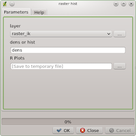
Now save the script. It will appear among other R scripts. Launch it and you will see this window:
script window
Script window
In 'layer' drop-down menu choose needed raster. In 'dens or hist' field type dens or hist to identify which representation of the raster cell data you prefer: density plot or a histogram. [ It would be great to know if it is possible to embed these options in drop-down menu as well (help me if you know how). ] In 'R plots' field set the destination of the graph to be saved (optional). If you chose density plot you will get something like this:
raster density plot
Density plot
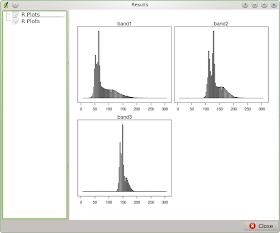
If you choose histogram, you will get something like this:
raster histogram
Histogram
And if you fail to provide correct value in 'dens or hist' field you will get this:
warning window
Fail window

How it works.

##layer=raster  provides us with the drop-down menu to select needed raster and it will be addresed as layer in our script. ##Tools=group will assign our script to the Tools group of R scripts in SEXTANTE. ##dens_or_hist=string provides us with the string input field dens or hist. ##showplots will show the plot in Results window after execution. library('rpanel') this library is needed to show pop-up window with the error when the user fails to type 4 letters correctly. library('rasterVis') this library works on top of raster package and it is responsible for plotting our graphs. Then we define condition to pop up error window via rp.messagebox if the plot type is misspelled or missing. The following piece of code is interesting:
im <- stack(layer)
test <- try(nbands(im))
if (class(test) == 'try-error') {im <- raster(layer)}
In order to correctely process the raster we need to have a RasterStack class for multi-band raster or a RasterLayer class if the raster is single-banded. 'raster' package is a bit weird with its classes so there are even different functions for determination of the number of bands for different classes and types of rasters. So the code above is weird too))) We assume that the raster is multi-banded and create a RasterStack object. Then we check whether our guess was correct: if raster is actually single-banded we will have an error if we try to use nbands() function on it.  If it is the case - we will create RasterLayer object instead of RasterStack.
Finally, we transform our raster to the RasterStack object to be able to run either densityplot() or histogram() function.

Final notes

In a blink of an eye we were able to create quite handy tool to replace a long broken one. But there is the downside. This script won't be able to handle huge rasters - I wasn't able to process my IKONOS imagery where sides of the rasters exceeds 10000 pixels. Also I would not recommend to use in on a hyperspectral imagery with the dozens of bands because the process will run extremely sloooow (it will take hours and tons of RAM) and the result will be obviously unreadable.