In my previous post I described how to perform pan-sharpening using OrfeoToolbox and QGIS. This time I will show you how to do this in R. At the bottom you will find several functions I wrote on top of the 'raster' package that allow a convenient pan-sharpening in R.
Motivation
You may wonder why I even bothered myself with pan-sharpening in R when I already have a nice model for pan-sharpening in QGIS. See, one can't control the data-type of the imagery returned by pan-sharpening that involves OTB. This leads to some unpleasant consequences: during pan-sharpening one will get floating point pixel values even if in initial values were integers. So for example a 600 MiB multi-spectral imagery (with integer pixel values) after pan-sharpening will grow to 5.2 GB. But if we will change datatype of the resulting imagery to force it store only integers it size will be reduced from 5.2 to 2.8 GB which is a huge difference. 'raster' package in R allows to control output datatype. Plus using R you can play with different filtering options to play with.
The Theory
In OTB pan-sharpening is performed using following well-known formula:
Where i and j are pixels indices, PAN is the panchromatic image, XS is the multi-spectral image and PANsmooth is the panchromatic image smoothed with a kernel to fit the multi-spectral image scale.
We will implement exact the same approach using 'raster' package for R.
pan <- raster('pan.tif')
multi <- brick('multi.tif')
pansharp <- processingPansharp(pan, multi)
output_path <- 'path_and_filename_without_extention'
saveResult(pansharp, output_path)
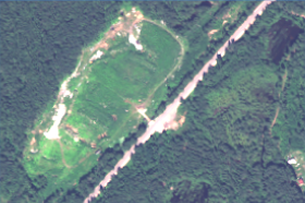
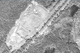
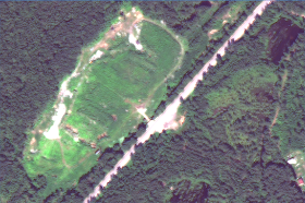
Here you are the example results from the script and from the OTB model for one of the illegal landfills in Russia:
We will implement exact the same approach using 'raster' package for R.
Code Usage and Result
As pan-sharpening is the type of procedure that will reoccur over some time I decided to write generic functions for pan-sharpening itself and for saving the results to have easier time in future.
The usage is as simple as:
pan <- raster('pan.tif')
multi <- brick('multi.tif')
pansharp <- processingPansharp(pan, multi)
output_path <- 'path_and_filename_without_extention'
saveResult(pansharp, output_path)
Here you are the example results from the script and from the OTB model for one of the illegal landfills in Russia:
 |
| Initial multi-band raster |
 |
| Initial panchromatic raster |
 |
| Result of pan-sharpening using R script |
 |
| Result of pan-sharpening using OTB |
Which output do you like better: from OTB or R? Comparing both output results you can notice that the output from R bears heavier filtering markings than the one from OTB. On the other hand R output has more hues of the green colours which actually helps in distinguishing different types of vegetation. As you will see in the code - one can easily adjust or modify procedure of filtering panchromatic raster (extractLPF() function) in order to get desired output.
The code
library(raster)


# Create needed functions -------------------------------------------------

pansharpFun <- function(raster){
    '
    This function pansharpens a raster
    '
    # @param raster - Raster object with 3 bands (to-be-pansharpened, high-res and low-frequency component of the high-res image)
    # @param band - band numver, integer
    # @return pansharpened_raster - pansharpened Raster object
    # pansharp = Lowres * Highres / LPF[Highres]

    pansharpened_raster <- (raster[,1] * raster[,2]) / raster[,3]
}

extractLPF <- function(pan, multi, filter = 'auto', fun = mean) {
    '
    Returns a low-frequency component of the high-resolution raster by the
        filter adjusted to the low-resolution raster
    '
    # @param pan - a high-resolution panchromatic raster - Raster object
    # @param multi - low-resolution raster to be pansharpened - Raster object
    # @param filter - a smoothing wondow - matrix
    # @param fun - a function to process filter (part of the focal() function)
    # @return LPF - a low-frequency component of the high-resolution raster - Raster object

    # Adjust filter size
    if (filter == 'auto') {
        pan_res <- res(pan) # (x, y) resolution of the panchromatic raster in CRS units (?)
        multi_res <- res(multi) # (x, y) resolution of the lowres raster in CRS units (?)
        x_res_ratio <- round(multi_res[1]/pan_res[1])
        y_res_ratio <- round(multi_res[2]/pan_res[2])
        total <- x_res_ratio + y_res_ratio
        filter <- matrix(1, nc = x_res_ratio, nr = y_res_ratio)

        # Enshure that the matrix has an uneven number of colums and rows (needed by focal())
        if (nrow(filter)%%2 == 0) {
            filter <- rbind(filter, 0)
        }
        if (ncol(filter)%%2 == 0) {
            filter <- cbind(filter, 0)
        }

    LPF <- focal(pan, w = filter, fun = fun) # low-frequency component

}


processingPansharp <- function(pan, multi, filter = 'auto', fun = mean){
    '
    Pansharpening routine
    '
    # @param pan - a high-resolution panchromatic raster - Raster object
    # @param multi - low-resolution raster to be pansharpened - Raster object
    # @param filter - a smoothing wondow - matrix
    # @param fun - a function to process filter (part of the focal() function)
    # @return pansharp - pansharpened 'multi' raster - Raster object

    # Check if input parameters are valid - we can loose a lot of time if some of the inputs is wrong

    LPF <- extractLPF(pan, multi, filter, fun)

    multi <- resample(multi, pan) # resample low-resolution image to match high-res one

    all <- stack(multi, pan, LPF)

    bands <- nbands(multi)
    pan_band <- bands + 1
    lpf_band <- bands + 2

    # Pansharpen layers from low-resolution raster one by one
    pansharp_bands <- list()
    for (band in 1:bands) {
        subset <- all[[c(band, pan_band, lpf_band)]]
        raster <- calc(subset, pansharpFun)
        pansharp_bands[[band]] <- raster
    }

    pansharp <- stack(pansharp_bands)
}

saveResult <- function(raster, path, format = 'GTiff', datatype = 'INT2S'){
    '
    Saves Raster object to location
    '
    # @param raster - raster to be saved - Raser object
    # @param path - path including filename without extention - string
    # @param format - format of the output raster accordingly to writeRaster() function - string
    # @param datatype - datatype of the raster accordingly to writeRaster() - string

    writeRaster(raster,
                path,
                format = format,
                datatype = datatype,
                overwrite = T)
}


# Do pansharpening --------------------------------------------------------


pan <- raster('pan.tif')
multi <- brick('multi.tif')
pansharp <- processingPansharp(pan, multi)
output_path <- 'r_pansharp-new' # includes path and filename but not the extention
saveResult(pansharp, output_path)
This is a really cool script. I am currently learning R and appreciate people that take the time and write scripts to do useful things that other GIS software packages can't always do.
ReplyDeleteThanks very much for this. What if my interest lies in pansharpening only in the G band and an infrared band (e.g., SWIR), e.g., for the calculation of a vegetative or water index? Is it as simple as substituting the bands of interest into the RasterBrick?
ReplyDeleteGreat script!!!, however, I found an error in your script. In line 69 you wrote "bands <- nbands(multi)", you must replace with "bands <- nlayers(multi)" otherwise you will get a raster brick with a single layer.
ReplyDeleteFinally, to get a great image with R I recommend to share this code:
fun <- function(x){
((x - minValue(x)) / (maxValue(x) - minValue(x)))*255
}
plotRGB(fun(pansharp), stretch = "lin")
Thanks for sharing this code, i have one question: what exactly the filter "auto" function does?
ReplyDelete